
MANOVA and Follow-Up ANOVAs
Synthetic methodological demonstration
Created from scratch with synthetic data and reconstructed context. No client data or original client document is used.
Analysis Plan
A one-way multivariate analysis of variance (MANOVA) was performed to determine whether the combined burnout profile differed across employment-hours bands. Employment-hours band was a five-level between-subjects factor coded as None, 1–10 hours, 11–20 hours, 21–30 hours, and 31+ hours. The dependent variables were Research Exhaustion, Research Cynicism, and Cognitive Weariness. In the GREPS measurement specification, these variables represent distinct first-order dimensions of Graduate Research Burnout; therefore, a multivariate group comparison was appropriate before conducting the outcome-specific follow-up tests.
The represented GREPS dataset contained 900 synthetic graduate-student records from 15 anonymous institutions and was cross-sectional and observational. Therefore, the case study describes differences and associations across employment-hours bands rather than causal effects of employment. Analyses were conducted in IBM SPSS Statistics. No covariates were included in the primary model because the stated case-study question required a direct one-factor group comparison. Institutional clustering was examined as a prespecified sensitivity issue.
Outcome Scoring and Analytic Sample
Before the inferential analyses were conducted, outcome scores were constructed from the original GREPS items. CYN4 and CW4 were reverse-coded as 8 minus the original response, while the original variables were retained unchanged. EXH_SCORE was calculated as the row mean of EXH1–EXH4; CYN_SCORE as the row mean of CYN1, CYN2, CYN3, and CYN4_R; and CW_SCORE as the row mean of CW1, CW2, CW3, and CW4_R. Consistent with the GREPS scoring rule for four-item scales, a score was calculated only when at least three of the four items were observed. Thus, all three composite scores remained on the original 1–7 response metric.
Before running the MANOVA, frequencies were reviewed for the employment-hours factor, and missingness was summarized for the grouping variable, source items, and three composite scores. Cases missing the grouping variable or any of the three final composite scores would have been excluded listwise from the multivariate model. Individual item values were not mean-imputed. Person-level mean scoring was applied only under the prespecified minimum-item rule defined in the GREPS analysis guide.
Research Hypotheses and Analysis Plan
Three prespecified outcome-level hypotheses were evaluated. A statistically significant omnibus MANOVA served as the multivariate gatekeeper before confirmatory interpretation of the three outcome-specific follow-up tests. The analysis first tested whether the vector of Exhaustion, Cynicism, and Cognitive Weariness differed across the five employment-hours bands while accounting for the correlations among the dependent variables (Rencher & Christensen, 2012).
Hypothesis 1
H1: Mean Research Exhaustion differs across employment-hours bands. This hypothesis was evaluated using the Exhaustion follow-up one-way ANOVA after the omnibus MANOVA. If the outcome-level omnibus test met the multiplicity-adjusted criterion, pairwise comparisons were used to determine which employment-hours bands differed.
Hypothesis 2
H2: Mean Research Cynicism differs across employment-hours bands. This hypothesis was evaluated using the Cynicism follow-up one-way ANOVA after the omnibus MANOVA. If the outcome-level omnibus test met the multiplicity-adjusted criterion, pairwise comparisons were used to determine which employment-hours bands differed.
Hypothesis 3
H3: Mean Cognitive Weariness differs across employment-hours bands. This hypothesis was evaluated using the Cognitive Weariness follow-up one-way ANOVA after the omnibus MANOVA. If the outcome-level omnibus test met the multiplicity-adjusted criterion, pairwise comparisons were used to determine which employment-hours bands differed.
Preliminary Screening and Assumption Assessment
Descriptive statistics will be produced for each outcome within each employment-hours band, including n, mean, standard deviation, standard error, range, and 95% confidence interval. Histograms, normal Q–Q plots, and boxplots will be examined within groups to identify substantial skew, tail problems, or unusual univariate observations. Scatterplot matrices and within-band correlations among the three outcomes will also be examined to assess approximate linear relationships and to ensure that the dependent variables are related without approaching singularity or extreme multicollinearity.
Multivariate outliers will be assessed within employment-hours bands using Mahalanobis distance based on the three dependent variables. A conservative chi-square criterion of p < .001 with 3 degrees of freedom (Mahalanobis D² > 16.266) will be used to flag cases for review. Flagged cases will be checked against the legal item ranges and will not be deleted solely because they are statistically unusual. The primary analyses will retain valid observations. If meaningful multivariate outliers are identified, the MANOVA will also be performed without the flagged cases as a sensitivity analysis, and any change in the substantive conclusions will be documented.
Homogeneity of covariance matrices will be examined using Box’s M test, whereas homogeneity of variance for each dependent variable will be assessed using Levene’s test. Because Box’s M is sensitive to departures from multivariate normality, the test will be treated as a diagnostic rather than an automatic pass/fail criterion. Group-size equality, distributional diagnostics, and the pattern of Levene tests will be considered together. Pillai’s trace will be used as the primary multivariate statistic because it is generally preferred when robustness to moderate assumption violations is important (Field, 2018; Rencher & Christensen, 2012).
Independence is supported at the respondent level because the dataset includes one record per student and contains no repeated measurements. However, the students are nested within 15 institutions. Therefore, institution-level dependence will be examined using random-intercept null models for the three outcomes. If the institutional intraclass correlations are nontrivial or the primary inference is sensitive to clustering, random-intercept mixed-model versions of the outcome-specific group comparisons will be reported as sensitivity analyses rather than replacing the prespecified MANOVA.
Primary MANOVA
A one-way MANOVA will be conducted in SPSS GLM with employment-hours band as the fixed factor and EXH_SCORE, CYN_SCORE, and CW_SCORE entered jointly as the dependent variables. The multivariate null hypothesis states that the population mean vector for the three burnout dimensions is equal across all five employment-hours bands. The omnibus familywise alpha level for the multivariate test will be .05.
Pillai’s trace will be used as the primary multivariate criterion. The results will be reported using Pillai’s V, the approximate F statistic, numerator and denominator degrees of freedom, p value, and partial eta squared where available. Wilks’ lambda, Hotelling’s trace, and Roy’s largest root will be retained in the SPSS output as supplementary diagnostics and will not be used to select the conclusion. A statistically significant Pillai test will be followed by the three prespecified outcome-level analyses.
Follow-Up ANOVAs and Post-Hoc Comparisons
For each dependent variable, SPSS will produce the conventional one-way ANOVA, Welch’s robust test, and the relevant homogeneity diagnostics. Because three outcome-level hypotheses will be tested after the MANOVA, a Bonferroni-adjusted alpha of .05/3 = .0167 will be applied to the three follow-up omnibus tests. This adjustment will be applied at the outcome level and will not replace the familywise adjustment incorporated in the selected post-hoc procedure.
If Levene’s test for an outcome is not statistically significant and the distributional diagnostics are acceptable, the standard one-way ANOVA F test will be used as the primary follow-up test, followed by Tukey’s honestly significant difference test for all pairwise band comparisons. If Levene’s test indicates heterogeneous variances, Welch’s ANOVA will be used for inference, followed by Games–Howell pairwise comparisons because this procedure is designed for unequal variances and unequal group sizes (Games & Howell, 1976). Brown–Forsythe output will be retained as an additional robust diagnostic.
Post-hoc comparisons will be interpreted only for outcomes whose omnibus follow-up test meets the adjusted .0167 criterion. For each supported outcome-level hypothesis, the final results will report group means and standard deviations, the selected omnibus statistic and degrees of freedom, p value, an effect-size estimate, and statistically significant pairwise mean differences with 95% confidence intervals. Partial eta squared from the GLM output will be reported as the principal omnibus effect-size measure. With a single between-subjects factor and no covariates, this value corresponds to the proportion of outcome variance attributable to employment-hours band relative to that factor and error.
If severe distributional problems remain after inspection, a Kruskal–Wallis test will be conducted for each outcome as a nonparametric sensitivity analysis. This analysis will not replace the MANOVA framework because it does not provide a single multivariate test of the three outcomes. Rather, it will be used to determine whether the substantive pattern of group differences is broadly dependent on the parametric assumptions.
Decision Rules for the Three Hypotheses
The confirmatory analyses will follow a consistent decision sequence. First, the omnibus Pillai MANOVA must be statistically significant at alpha = .05. Second, H1, H2, and H3 will each be evaluated using the corresponding follow-up omnibus test at alpha = .0167. A hypothesis will be considered supported only when its outcome-level omnibus test meets this criterion; the post-hoc results will then identify the specific employment-hours bands responsible for the overall difference. An isolated statistically significant pairwise comparison will not be considered support when the corresponding outcome-level omnibus test does not meet the prespecified criterion.
SPSS values displayed as .000 will be reported as p < .001 rather than p = .000. All other exact p values will be reported to three decimal places, together with confidence intervals and effect sizes, so that interpretation is not based on statistical significance alone. The supplied syntax retains all valid cases in the primary analysis and clearly distinguishes the optional sensitivity analyses for multivariate outliers, nonnormality, and institution clustering.
Findings
Analytic Sample, Scoring, and Scale Quality
All 900 records had a valid employment-hours band and valid scores for all three MANOVA outcomes after application of the minimum-item scoring rule. The five employment-hours bands included 223 students reporting no paid work outside the research role, 212 reporting 1–10 hours, 219 reporting 11–20 hours, 136 reporting 21–30 hours, and 110 reporting 31 or more hours. For Exhaustion, Cynicism, and Cognitive Weariness, respectively, 28, 20, and 22 records contained three observed source items rather than four; all remaining records contained four observed items. Because these cases satisfied the prespecified three-of-four item rule, all 900 cases were retained in the primary MANOVA (N = 900).
The internal-consistency results were acceptable for each of the three four-item scales. Cronbach's alpha was .825 for Research Exhaustion, .814 for Research Cynicism, and .796 for Cognitive Weariness. These analyses were considered supplemental checks of scale quality rather than hypothesis tests.
Table 1
Descriptive statistics by employment-hours band
| Employment-hours band | n | Exhaustion M (SD) | Cynicism M (SD) | Cognitive Weariness M (SD) |
|---|---|---|---|---|
| None | 223 | 3.52 (1.29) | 3.56 (1.33) | 3.54 (1.29) |
| 1–10 hours | 212 | 3.71 (1.34) | 3.36 (1.20) | 3.59 (1.27) |
| 11–20 hours | 219 | 3.98 (1.35) | 3.64 (1.39) | 3.74 (1.33) |
| 21–30 hours | 136 | 4.34 (1.23) | 3.80 (1.30) | 3.95 (1.28) |
| 31+ hours | 110 | 4.59 (1.31) | 3.97 (1.41) | 4.26 (1.30) |
Note. Scores are means on the original 1–7 metric. M = mean; SD = standard deviation.
Assessment of MANOVA Assumptions
The within-band histograms, normal Q–Q plots, and boxplots were examined for each dependent variable. The distributions were broadly symmetric, and the Q–Q plots followed the reference line reasonably well, with no pattern indicating severe nonnormality. The boxplots also indicated broadly comparable spread across the employment-hours bands. Figures 1 through 3 are reserved for the three outcome boxplots, whereas Figures 4 through 6 provide a compact presentation of Normal Q–Q plots for the residuals from the three one-way follow-up models.
Figure 1
Boxplots of Exhaustion across employment-hours bands
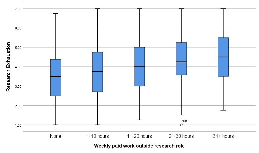
Figure 2
Boxplots of Cynicism across employment-hours bands
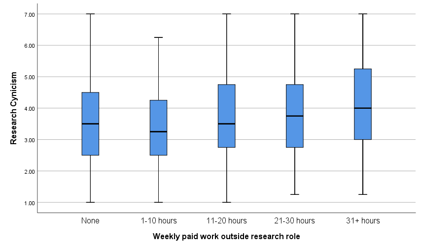
Figure 3
Boxplots of Cognitive Weariness across employment-hours bands
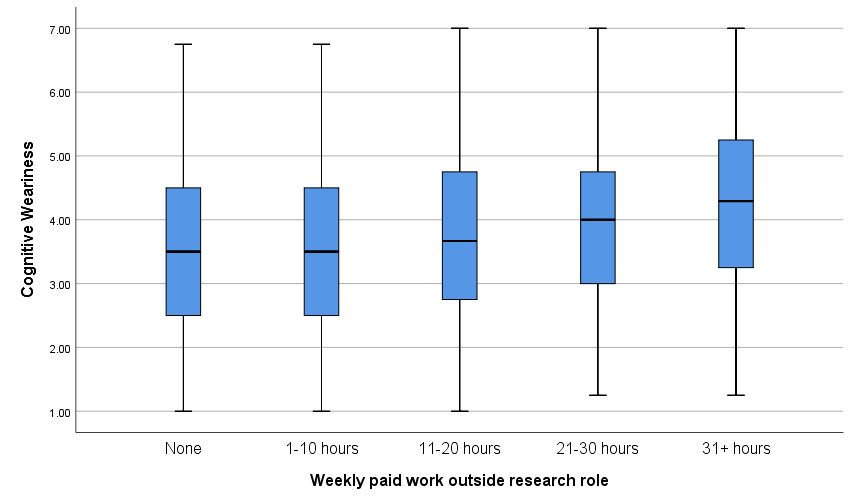
Figure 4
Normal Q–Q plots of the one-way follow-up model for Exhaustion ANOVA residuals
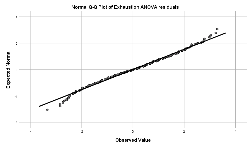
Figure 5
Normal Q–Q plots of the one-way follow-up model for Cynicism ANOVA residuals
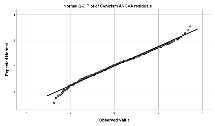
Figure 6
Normal Q–Q plots of the one-way follow-up model for Cognitive Weariness ANOVA residuals
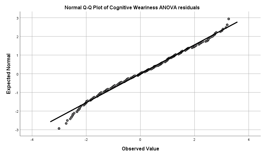
The within-band Mahalanobis-distance analysis identified no multivariate outliers at the prespecified p < .001 criterion (D² > 16.266); therefore, all 900 cases were retained. Box’s test was not statistically significant, Box’s M = 34.644, F = 1.432, p = .078, indicating no evidence that the covariance matrices differed across groups. Levene’s tests based on the mean were also nonsignificant for Exhaustion, F(4, 895) = 0.796, p = .528, Cynicism, F(4, 895) = 1.340, p = .253, and Cognitive Weariness, F(4, 895) = 0.189, p = .944. Taken together with the distributional diagnostics, these results indicated that the assumptions were sufficiently reasonable for the planned Pillai MANOVA and conventional follow-up ANOVAs.
Results of the Omnibus MANOVA
The results of the one-way MANOVA revealed a statistically significant multivariate difference in the combined profile of Research Exhaustion, Research Cynicism, and Cognitive Weariness across the five employment-hours bands, Pillai’s V = .083, F(12, 2685) = 6.356, p < .001, partial η² = .028. Thus, the multivariate gatekeeper criterion was met, and the three prespecified outcome-level hypotheses were evaluated using follow-up one-way ANOVAs.
Table 2
Omnibus MANOVA and homogeneity diagnostics
| Test | Statistic | df | p-value | Effect size |
|---|---|---|---|---|
| Pillai’s trace | V = .083; F = 6.356 | 12, 2685 | < .001 | Partial η² = .028 |
| Box’s M | M = 34.644; F = 1.432 | 24, 1,235,628.489 | .078 | — |
| Levene: Exhaustion | F = 0.796 | 4, 895 | .528 | — |
| Levene: Cynicism | F = 1.340 | 4, 895 | .253 | — |
| Levene: Cognitive Weariness | F = 0.189 | 4, 895 | .944 | — |
Note. Pillai’s trace was the prespecified primary multivariate statistic. SPSS values displayed as .000 are reported as p < .001.
Follow-Up ANOVAs
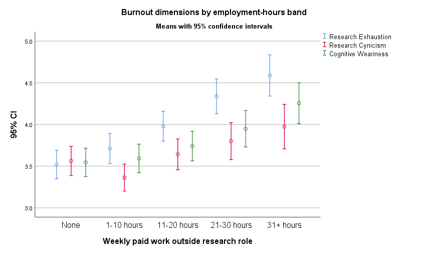
Because the omnibus MANOVA was statistically significant, one-way ANOVAs were conducted for the three dependent variables. The prespecified Bonferroni-adjusted criterion for these three confirmatory tests was α = .0167. The results showed that all three follow-up ANOVAs met this criterion. The overall pattern of group means and the corresponding 95% confidence intervals are reserved for presentation in Figure 7.
Table 3
Follow-up one-way ANOVAs by outcome
| Outcome | F | df | p-value | Partial η² | Decision at α = .0167 |
|---|---|---|---|---|---|
| Research Exhaustion | 17.288 | 4, 895 | < .001 | .072 | Significant |
| Research Cynicism | 4.729 | 4, 895 | .001 | .021 | Significant |
| Cognitive Weariness | 7.170 | 4, 895 | < .001 | .031 | Significant |
Note. Partial η² values are from the SPSS GLM follow-up tests. All three outcome-level tests met the prespecified Bonferroni-adjusted criterion of .0167.
Figure 7
Mean burnout-dimension scores by employment-hours band with 95% confidence intervals
Hypothesis 1
Hypothesis 1 predicted that mean Research Exhaustion would differ across employment-hours bands. The results of the follow-up ANOVA revealed a statistically significant difference in Research Exhaustion across the employment-hours bands, F(4, 895) = 17.288, p < .001, partial η² = .072. Mean Exhaustion increased from 3.52 in the no-paid-work group to 4.59 in the 31+ hours group. Tukey HSD comparisons indicated higher Exhaustion for the 11–20 hour group than the no-work group, for the 21–30 hour group than the no-work and 1–10 hour groups, and for the 31+ hour group than the no-work, 1–10 hour, and 11–20 hour groups. No other Tukey-adjusted pairwise comparisons were statistically significant. Accordingly, Hypothesis 1 was supported.
Hypothesis 2
Hypothesis 2 predicted that mean Research Cynicism would differ across employment-hours bands. The results of the follow-up ANOVA revealed a statistically significant difference in Research Cynicism across the employment-hours bands, F(4, 895) = 4.729, p = .001, partial η² = .021. Cynicism was lowest in the 1–10 hour group (M = 3.36) and highest in the 31+ hour group (M = 3.97). Tukey HSD comparisons indicated that the 21–30 hour group had higher Cynicism than the 1–10 hour group and that the 31+ hour group also had higher Cynicism than the 1–10 hour group. No other Tukey-adjusted pairwise comparisons were statistically significant. Accordingly, Hypothesis 2 was supported.
Hypothesis 3
Hypothesis 3 predicted that mean Cognitive Weariness would differ across employment-hours bands. The results of the follow-up ANOVA revealed a statistically significant difference in Cognitive Weariness across the employment-hours bands, F(4, 895) = 7.170, p < .001, partial η² = .031. Mean Cognitive Weariness increased from 3.54 in the no-paid-work group to 4.26 in the 31+ hours group. Tukey HSD comparisons indicated higher Cognitive Weariness for the 21–30 hour group than the no-work group and for the 31+ hour group than the no-work, 1–10 hour, and 11–20 hour groups. The remaining pairwise comparisons were not statistically significant after Tukey adjustment. Accordingly, Hypothesis 3 was supported.
Table 4
Statistically significant Tukey HSD pairwise comparisons
| Outcome | Higher-hours band | Lower-hours band | Mean difference | 95% CI | p-value |
|---|---|---|---|---|---|
| Exhaustion | 11–20 hours | None | .460 | [.119, .801] | .002 |
| Exhaustion | 21–30 hours | None | .820 | [.430, 1.209] | < .001 |
| Exhaustion | 31+ hours | None | 1.069 | [.652, 1.486] | < .001 |
| Exhaustion | 21–30 hours | 1–10 hours | .627 | [.233, 1.020] | < .001 |
| Exhaustion | 31+ hours | 1–10 hours | .876 | [.456, 1.297] | < .001 |
| Exhaustion | 31+ hours | 11–20 hours | .609 | [.191, 1.028] | .001 |
| Cynicism | 21–30 hours | 1–10 hours | .437 | [.040, .835] | .022 |
| Cynicism | 31+ hours | 1–10 hours | .611 | [.187, 1.036] | .001 |
| Cognitive Weariness | 21–30 hours | None | .404 | [.019, .789] | .035 |
| Cognitive Weariness | 31+ hours | None | .710 | [.298, 1.123] | < .001 |
| Cognitive Weariness | 31+ hours | 1–10 hours | .663 | [.247, 1.078] | < .001 |
| Cognitive Weariness | 31+ hours | 11–20 hours | .514 | [.101, .928] | .006 |
Note. Mean differences are presented as the higher-hours band minus the lower-hours band. Confidence intervals and p values are Tukey HSD adjusted within each outcome. Post-hoc tests were interpreted only after the corresponding outcome-level omnibus test met α = .0167.
Sensitivity Analyses
The results of the nonparametric sensitivity analyses were consistent with the primary parametric findings. Kruskal–Wallis tests revealed statistically significant differences for Exhaustion, H(4) = 61.627, p < .001, Cynicism, H(4) = 15.805, p = .003, and Cognitive Weariness, H(4) = 27.899, p < .001. Because no case exceeded the prespecified multivariate-outlier threshold, the outlier-excluded MANOVA was identical to the primary MANOVA.
Institution-level random-intercept null models indicated negligible clustering, with estimated ICCs of approximately .002 for Exhaustion, .000 for Cynicism, and .008 for Cognitive Weariness. The Cynicism null model and the optional fixed-effect mixed models for Exhaustion and Cynicism produced non-positive-definite Hessian or boundary warnings because the institution-level variance was estimated at or extremely close to zero. Therefore, these warned models were not used for inference. Given the trivial ICCs, the prespecified condition for relying on cluster-aware outcome-specific sensitivity models was not met, and the conclusions from the primary MANOVA and ANOVAs were retained.
Summary of Results
The synthetic GREPS data revealed a statistically significant multivariate association between employment-hours band and the combined burnout profile of Research Exhaustion, Research Cynicism, and Cognitive Weariness. Pillai’s trace was statistically significant, and all three prespecified follow-up ANOVAs met the Bonferroni-adjusted outcome-level criterion. Accordingly, Hypotheses 1, 2, and 3 were supported.
The strongest pattern was observed for Research Exhaustion, which had the largest outcome-specific effect (partial η² = .072) and increased progressively across the employment-hours bands. Cognitive Weariness also tended to be higher in the heavier employment bands, with the 31+ hour group exceeding the three lowest bands. Research Cynicism showed a smaller overall effect (partial η² = .021), with the most reliable pairwise differences involving the 1–10 hour group, which had lower Cynicism than the 21–30 and 31+ hour groups. The nonparametric sensitivity analyses produced the same overall group-difference conclusions, no multivariate outliers were identified, and the institution-level ICCs were negligible.
These findings represent a methodological demonstration based entirely on synthetic data. Therefore, they should not be interpreted as evidence that paid employment causes burnout among real graduate students or as population estimates for graduate students or universities.
References
Field, A. (2018). Discovering statistics using IBM SPSS Statistics (5th ed.). SAGE Publications.
Games, P. A., & Howell, J. F. (1976). Pairwise multiple comparison procedures with unequal N’s and/or variances: A Monte Carlo study. Journal of Educational Statistics, 1(2), 113–125. https://doi.org/10.3102/10769986001002113
Graduate Research Engagement and Persistence Study (GREPS): Data cleaning, scoring, validation, and analysis guide (Version 1.0). (2026). [Unpublished technical documentation].
Graduate Research Engagement and Persistence Study (GREPS): Methodology and study specification (Version 1.0). (2026). [Unpublished technical documentation].
IBM Corp. (n.d.). PRINT subcommand (GLM: Multivariate command). IBM Documentation. Retrieved August 17, 2026, from https://www.ibm.com/docs/en/spss-statistics/32.0.0?topic=multivariate-print-subcommand-glm-command
IBM Corp. (n.d.). STATISTICS subcommand (ONEWAY command). IBM Documentation. Retrieved August 17, 2026, from https://www.ibm.com/docs/en/spss-statistics/32.0.0?topic=oneway-statistics-subcommand-command
Rencher, A. C., & Christensen, W. F. (2012). Methods of multivariate analysis (3rd ed.). Wiley. https://doi.org/10.1002/9781118391686
Need help with a similar research question?
Share a short, non-confidential summary of your study and the decision you need to make.